

DataOps: Apache Spark - Intermediate (Part 1)
A practical approach toward learning data science with the help of PySpark. Part 1: RDDs and DataFrames.

I'm a senior full-stack developer, and I love software engineering. I believe by working together we can create wonderful assets for the world, and we can shape the future as we shape our own destiny, and no goal is too ambitious. 💫 I try to be optimistic and energetic, and I'm always open to collaboration. 👥 Contact me if you have something on your mind and let's see where it goes 🚀
Overview
In a previous article, we covered the basics of Apache Spark. Now that the foundational concepts and workflow architecture of the spark are covered, we'll be exploring PySpark and its conventional practices, and implementations.
PySpark has the following core modules:
PySpark RDD (pyspark.RDD)
PySpark DataFrame and SQL (pyspark.sql)
PySpark Streaming (pyspark.streaming)
PySpark MLib (pyspark.ml, pyspark.mllib)
PySpark GraphFrames (GraphFrames)
PySpark Resource (pyspark.resource) (Only in PySpark 3.0+)
You can also find other Python packages and modules at spark-packages.org.
Resilient Distributed Dataset(RDD)
Introduction
RDD (Resilient Distributed Dataset) is a fundamental building block of PySpark which is a fault-tolerant, immutable distributed collection of objects. Each record in RDD is divided into logical partitions, which can be computed on different nodes of the cluster.
More or less, we can regard them as other python lists where the implementation of distributed computation strategies is handled internally by Spark.
Resilience or Fault-tolerance means in case of node failures, with the help of RDD lineage graph (DAG) Spark will be able to recompute missing or damaged partitions.
By default, RDDs are stored in-memory but Spark will store them on disk in case RAM is overloaded. However, users can also explicitly store RDDs by the persist method on the disk or other storage strategies. To keep the computation speed as fast as possible, the DAGScheduler places the data partitions in such a way that the task is close to the data as much as possible.
Difference with DSM
Distributed Shared Memory is a common memory data abstraction. In DSM, applications can read and write to any location in the global address space. Spark strategy for handling RDD is different from DSM in the following manners:
| Feature | DSM | RDD |
| Write Operations | Fine-Grained | Coarse-Grained |
| Read Operations | Fine-Grained | Coarse- and Fine-Grained |
| Consistency | "Developer Strategy"-Dependant | High due to immutability |
| Fault Tolerance | "Developer Strategy"-Dependant | Lineage DAG of Immutable RDDs |
| Speculative Execution* | Not Supported | Supported |
| At RAM Overload | Performance is impacted | Excess is stored on disk |
Now let's go through a couple of technical terms in the comparative table above.
X-Grained
Fine-Grained means individual elements can be queried/accessed/transformed, while Coarse-Grained means only the whole dataset is available for such operations.
Speculative Execution
Apache Spark has the ‘speculative execution’ feature to handle the slow tasks in a stage due to environment issues like slow network, disk etc. If one task is running slowly in a stage, Spark driver can launch a speculation task for it on a different host. Between the regular task and its speculation task, Spark system will later take the result from the first successfully completed task and kill the slower one.
When to Use
When dealing with unstructured data like text and media streams, RDD has a higher performance. RDDs can work with and without a dataset schema.
Code-Wise Implementation
Initialization
# Running in spark/bin/pyspark
print(spark)
# <pyspark.sql.session.SparkSession object at 0x7fc4e9980490>
sc = spark.sparkContext
# 1. From a collection:
# ============================================================
a = range(0,10)
# array([0, 1, 2, 3, 4, 5, 6, 7, 8, 9])
rdd = sc.parallelize(a)
print(rdd)
# ParallelCollectionRDD[0] at readRDDFromFile at PythonRDD.scala:274

# You can't access RDDs elements by subscripting:
print(rdd[0])
# Traceback (most recent call last):
#   File "<stdin>", line 1, in <module>
# TypeError: 'RDD' object is not subscriptable

# In order to access the elements in an RDD you can use:
print(rdd.collect())
# [0, 1, 2, 3, 4, 5, 6, 7, 8, 9]
# ============================================================
# 2. From a text-based* file
# ============================================================
# PySpark can create distributed datasets from any storage source supported by Hadoop, including your local file system, HDFS, Cassandra, HBase, Amazon S3, etc. Spark supports text files, SequenceFiles, and any other Hadoop InputFormat.
# *: Text-based is a means to exclude big data file formats like sequence files, pickle files, and such.

# Text file RDDs can be created using SparkContext’s textFile method. This method takes a URI for the file (either a local path on the machine, or a hdfs://, s3a://, etc URI) and reads it as a collection of lines.

distFile = sc.textFile("/opt/spark-data/test.txt")
print(distFile)
# /opt/spark-data/test.txt MapPartitionsRDD[8] at textFile at NativeMethodAccessorImpl.java:0

# Now calling the `collect` will return an ordered collection of the lines in the file.
print(distFile.collect())
# ['Hello my name is Andrew!', 'This is a sample for demonstrating spark distributed processing of a file.', 'This is a sample for demonstrating spark distributed processing of a file.', 'This is a sample for demonstrating spark distributed processing of a file.']
# ============================================================
# 3. From a directory
# ============================================================
# Using `wholeTextFiles` will return an array of (key, value) tuples where keys are the full access path of each file and values are the content of each.
files = sc.wholeTextFiles("/opt/spark-data")
print(files.collect())
# [('file:/opt/spark-data/test.txt', 'Hello my name is Andrew!\r\nThis is a sample for demonstrating spark distributed processing of a file.\r\nThis is a sample for demonstrating spark distributed processing of a file.\r\nThis is a sample for demonstrating spark distributed processing of a file.'), ('file:/opt/spark-data/test2.txt', 'This is another test file'), ('file:/opt/spark-data/user_info.csv', 'id,username\r\n1,Amir\r\n2,Sepideh\r\n')]
Single Operators
(Involving a single RDD)
Arithmetics
# By executing the following tasks, spark will submit the workload to the designated available workers and return the result:
print(rdd.mean())
# 4.5
print(rdd.min())
# 0
print(rdd.max())
# 9
Member Access
# ============================================================
# You can change RDD elements using `map` and `reduce`; for example:
# Let's try and find the occurancy rate of letter `A` in `distFile`.
# First, let's find the number of times that letter 'a' or 'A' was repeated.
import re
def a_count(str: string):
    return len(re.findall(r'a|A', str))

total_a = distFile.map(a_count).reduce(lambda a, b: a + b)
print(total_a)
# 17

# Now let's find the total number of characters in the `distFile`:
total_char = distFile.map(lambda line: len(line)).reduce(lambda a, b: a + b)
print(total_char)
# 246

# Finally we divide them and calculate the percentage:
print("%.2f%%" % ((total_a * 100) / total_char))
# 6.91%
# ============================================================
# Another fine-grained access method is `foreach` which performs a certain method for each element of the RDD collection WITHOUT CHANGING IT like `map`.
# For example, let's print each element of the collection:
rdd.foreach(print)
# 0
# 1
# 6
# 4
# 7
# 2
# 5
# 3
# 9
# 8

# As you can see, the elements were printed in arbiterary order. This is because RDDs are distributed over different partitions and workers, hence if not explicitly specified, the order by which spark accesses these elements will most probably not be in the order of the original collection.
# ============================================================
# In order to access members based on a condition, you can use `filter` by passing a boolean returning function:
rdd.filter(lambda x: x % 2 == 0).collect()
# [0, 2, 4, 6, 8]
# ============================================================
# There's also `reduceByKey`, `groupByKey` that can be used for Paired-RDDs*:
paired = rdd.map(lambda x: (x % 3, x**2))
print(paired.collect())
# [(0, 0), (1, 1), (2, 4), (0, 9), (1, 16), (2, 25), (0, 36), (1, 49), (2, 64), (0, 81)]
paired.reduceByKey(lambda x, y: x + y).collect()
# [(0, 126), (1, 66), (2, 93)]

paired.groupByKey().collect()
# [(0, <pyspark.resultiterable.ResultIterable object at 0x7f5035a090d0>), (1, <pyspark.resultiterable.ResultIterable object at 0x7f5035a091d0>), (2, <pyspark.resultiterable.ResultIterable object at 0x7f5035b8a850>)]
temp = paired.groupByKey().collect()
for k, v in temp:
    print(k, list(v))
# 0 [0, 9, 36, 81]
# 1 [1, 16, 49]
# 2 [4, 25, 64]

paired.countByKey()
# defaultdict(<class 'int'>, {0: 4, 1: 3, 2: 3})
paired.countByKey().items()
# dict_items([(0, 4), (1, 3), (2, 3)])
Note: Paired-RDDs are just RDDs containing KVPs (Key - Value Paired Data) as tuples.
Persistence
There are two approaches to the persistence of RDDs in Spark:
Caching
Called by
rdd.cache()orrdd.persist():Persisting or caching with
StorageLevel.DISK_ONLYcause the generation of RDD to be computed and stored in a location such that subsequent use of that RDD will not go beyond that point in recomputing the lineage.After persist is called, Spark still remembers the lineage of the RDD even though it doesn't call it.
Secondly, after the application terminates, the cache is cleared and file is destroyed.
Checkpointing
Called by
rdd.localCheckpoint()andrdd.checkpoint()Checkpointing stores the RDD physically to HDFS (requires distributed storage) and destroys the lineage that created it.
The checkpoint file won't be deleted even after the Spark application is terminated.
Checkpoint files can be used in subsequent job runs or driver programs.
Checkpointing an RDD causes double computation because the operation will first call a cache before doing the actual job of computing and writing to the checkpoint directory.
(Source)
Q: What kind of RDD needs to be cached ?
Those which will be repeatedly computed and are not too large.
Q: What kind of RDD needs checkpoint ?
the computation takes a long time
the computing chain is too long
depends too many RDDs
Actually, saving the output of
ShuffleMapTaskon local disk is alsocheckpoint, but it is just for data output of partition.Q: When to checkpoint ?
As mentioned above, every time a computed partition needs to be cached, it is cached into memory. However,
checkpointdoes not follow the same principle. Instead, it waits until the end of a job, and launches another job to finishcheckpoint. An RDD which needs to be checkpointed will be computed twice; thus it is suggested to do ardd.cache()beforerdd.checkpoint(). In this case, the second job will not recompute the RDD. Instead, it will just read cache. In fact, Spark offersrdd.persist(StorageLevel.DISK_ONLY)method, like caching on disk. Thus, it caches RDD on disk during its first computation, but this kind ofpersistandcheckpointare different, we will discuss the difference later.(Source)
I highly suggest referring to the source mentioned in the quote for an in-depth guide.
For caching, there are different storage level configurations that one can use by passing an instance of pyspark.StorageLevel class or by passing a predefined config which are the attributes of the same class. A list is available in the official docs.
# 1. Caching
# ============================================================
# One can use `persist` or `cache` to save an RDD for later recall.
rdd.persist()
# ============================================================
# 2. Checkpointing
# ============================================================
# Local checkpoint stores your data in executors storage (as shown in your screenshot). It is useful for truncating the lineage graph of an RDD, however, in case of node failure you will lose the data and you need to recompute it (depending on your application you may have to pay a high price).
# 'Standard' checkpoint stores your data in a reliable file system (like hdfs). It is more expensive to perform but you will not need to recompute the data even in case of failures. Of course, it truncates the lineage graph.
# Truncating a long lineage graph avoid getting is particularly useful in iterative algorithms

rdd.localCheckpoint()
rdd.isCheckpointed()
# False
rdd.isLocallyCheckpointed()
# True
To DataFrame
You can turn RDDs into DataFrames (and vice-versa), but you have got to format the RDD elements in a comprehensive way for Spark to successfully pick up what you mean by the transformation from a schema-less data structure to a schema-full one.
# Consider the following case
rdd_t = sc.parallelize(a)
print(rdd.collect())
# [0, 1, 2, 3, 4, 5, 6, 7, 8, 9]
rdd_t.toDF()
# ValueError: The first row in RDD is empty, can not infer schema
The error above is because Spark doesn't understand how you want to distribute the flat data into a tabular one. If you want each element to be a single row then you can:
rdd_t2 = rdd_t.map(lambda x: (x,))
rdd_t2.collect()
# [(0,), (1,), (2,), (3,), (4,), (5,), (6,), (7,), (8,), (9,)]
rdd_t2.toDF().show()
# +---+
# | _1|
# +---+
# |  0|
# |  1|
# |  2|
# |  3|
# |  4|
# |  5|
# |  6|
# |  7|
# |  8|
# |  9|
# +---+

# You can also specify the schema you wish to apply to each column (each element of each tuple)
rdd_t2.toDF(schema=['user_id']).show()
# +-------+
# |user_id|
# +-------+
# |      0|
# |      1|
# |      2|
# |      3|
# |      4|
# |      5|
# |      6|
# |      7|
# |      8|
# |      9|
# +-------+
Repartitioning & Coalescing
repartition() is used to increase or decrease the RDD/DataFrame partitions whereas the PySpark coalesce() is used to only decrease the number of partitions in an efficient way. Both are very expensive operations as they shuffle the data across many partitions hence try to minimize using these as much as possible.
print(rdd_t.getNumPartitions())
# 4
# The default value for the number of partitions is set to the number of all cores on all nodes in a cluster, on local, it is set to the number of cores on your system, that is dedicated to the spark containerized application; in my case, I only allocated 4 CPU cores to my Docker setup, hence default value in my local is 4.

# `glom` method will collect the data stored in each partition and coalesces them in one array/list:
print(rdd_t.glom().collect())
# [[0, 1], [2, 3, 4], [5, 6], [7, 8, 9]]

repartitioned_rdd_t = rdd_t.repartition(3)
print(repartitioned_rdd_t.glom().collect())
# [[], [0, 1, 5, 6], [2, 3, 4, 7, 8, 9]]

coalesced = rdd.coalesce(3)
coalesced.glom().collect()
# [[0, 1], [2, 3, 4], [5, 6, 7, 8, 9]]

# Notice that after the `coalesce` method, only the 4th partitioned is merged with the 3rd partition, and the rest is left as they are. However, after `repartition` all partitions are changed.

# On a side-note, it's pretty normal for some partitions to be left empty in Spark. This is because of some modulo and hashing operation during shuffling of partitions.
You can also change the default partition count of the shuffle operation by
# Setting default shuffle count for RDDs
spark.conf.set("spark.default.parallelism",100)

# Setting default shuffle count for DataFrames
spark.conf.set("spark.sql.shuffle.partitions",100)
What should I set the default shuffling count to?
Based on your dataset size, a number of cores, and memory, Spark shuffling can benefit or harm your jobs. When you dealing with less amount of data, you should typically reduce the shuffle partitions otherwise you will end up with many partitioned files with less number of records in each partition. which results in running many tasks with lesser data to process.
On other hand, when you have too much of data and having less number of partitions results in fewer longer running tasks and some times you may also get out of memory error.
Getting a right size of the shuffle partition is always tricky and takes many runs with different value to achieve the optimized number. This is one of the key property to look for when you have performance issues on Spark jobs.
Sequence Files
Sequence files are a special kind of file format in a Big data environment, which are used to read or write data in binary types from or to a file. Using PySpark, you can write Paired-RDDs.
# We can't use `np.arange`. More info here: https://stackoverflow.com/questions/75840771/how-to-save-a-paired-rdd-as-a-sequence-file-in-pyspark
a = range(100)
print(a)
# array([ 0,  1,  2,  3,  4,  5,  6,  7,  8,  9, 10, 11, 12, 13, 14, 15, 16,
#       17, 18, 19, 20, 21, 22, 23, 24, 25, 26, 27, 28, 29, 30, 31, 32, 33,
#       34, 35, 36, 37, 38, 39, 40, 41, 42, 43, 44, 45, 46, 47, 48, 49, 50,
#       51, 52, 53, 54, 55, 56, 57, 58, 59, 60, 61, 62, 63, 64, 65, 66, 67,
#       68, 69, 70, 71, 72, 73, 74, 75, 76, 77, 78, 79, 80, 81, 82, 83, 84,
#       85, 86, 87, 88, 89, 90, 91, 92, 93, 94, 95, 96, 97, 98, 99])

rdd = sc.parallelize(a)
# turn into a list of tuples so that it can be interpreted as (key, value) pairs (KVP) for saving it as a sequenceFile
rdd.map(lambda x: (x, x**2)).saveAsSequenceFile("/opt/spark-data/saved-rdd")

# Now let's load the file to see if we can retrieve the correct results
rdd2 = sc.sequenceFile("/opt/spark-data/saved-rdd")
print(rdd2.collect())
# [(0, 0), (1, 1), (2, 4), (3, 9), (4, 16), (5, 25), (6, 36), (7, 49), (8, 64), (9, 81), (10, 100), (11, 121), (12, 144), (13, 169), (14, 196), (15, 225), (16, 256), (17, 289), (18, 324), (19, 361), (20, 400), (21, 441), (22, 484), (23, 529), (24, 576), (25, 625), (26, 676), (27, 729), (28, 784), (29, 841), (30, 900), (31, 961), (32, 1024), (33, 1089), (34, 1156), (35, 1225), (36, 1296), (37, 1369), (38, 1444), (39, 1521), (40, 1600), (41, 1681), (42, 1764), (43, 1849), (44, 1936), (45, 2025), (46, 2116), (47, 2209), (48, 2304), (49, 2401), (50, 2500), (51, 2601), (52, 2704), (53, 2809), (54, 2916), (55, 3025), (56, 3136), (57, 3249), (58, 3364), (59, 3481), (60, 3600), (61, 3721), (62, 3844), (63, 3969), (64, 4096), (65, 4225), (66, 4356), (67, 4489), (68, 4624), (69, 4761), (70, 4900), (71, 5041), (72, 5184), (73, 5329), (74, 5476), (75, 5625), (76, 5776), (77, 5929), (78, 6084), (79, 6241), (80, 6400), (81, 6561), (82, 6724), (83, 6889), (84, 7056), (85, 7225), (86, 7396), (87, 7569), (88, 7744), (89, 7921), (90, 8100), (91, 8281), (92, 8464), (93, 8649), (94, 8836), (95, 9025), (96, 9216), (97, 9409), (98, 9604), (99, 9801)]
Note
- If you have a lot of small-sized files then it will be very inefficient to read all of them. If you are using a Hadoop job then it will be most inefficient. Your record reader will have to read all the files one by one and for each file one mapper will be needed. This will use lots of resources of the cluster unnecessarily. To solve this we can create a large file out of the small files. If we create a sequence file out of these small files, then it will allow the dataset to be splitted. So sequence files will be one of the solutions to overcome small files problem in Spark or Hadoop.
Pickle Files
A quick introduction to pickle files in Python:
Pickle Files
In this section, we will introduce another way to store the data to the disk - pickle. We talked about saving data into text file or csv file. But in certain cases, we want to store dictionaries, tuples, lists, or any other data type to the disk and use them later or send them to some colleagues. This is where pickle comes in, it can serialize objects so that they can be saved into a file and loaded again later.
Pickle can be used to serialize Python object structures, which refers to the process of converting an object in the memory to a byte stream that can be stored as a binary file on disk. When we load it back to a Python program, this binary file can be de-serialized back to a Python object.
While saving to a pickle file, we don't need to adhere to a KVP data format.
a = range(100)
print(a)
# array([0, 1, 2, 3, 4, 5, 6, 7, 8, 9, 10, 11, 12, 13, 14, 15, 16, 17, 18, 19, 20, 21, 22, 23, 24, 25, 26, 27, 28, 29, 30, 31, 32, 33, 34, 35, 36, 37, 38, 39, 40, 41, 42, 43, 44, 45, 46, 47, 48, 49, 50, 51, 52, 53, 54, 55, 56, 57, 58, 59, 60, 61, 62, 63, 64, 65, 66, 67, 68, 69, 70, 71, 72, 73, 74, 75, 76, 77, 78, 79, 80, 81, 82, 83, 84, 85, 86, 87, 88, 89, 90, 91, 92, 93, 94, 95, 96, 97, 98, 99])

rdd = sc.parallelize(a)
print(rdd.collect())
# [0, 1, 2, 3, 4, 5, 6, 7, 8, 9, 10, 11, 12, 13, 14, 15, 16, 17, 18, 19, 20, 21, 22, 23, 24, 25, 26, 27, 28, 29, 30, 31, 32, 33, 34, 35, 36, 37, 38, 39, 40, 41, 42, 43, 44, 45, 46, 47, 48, 49, 50, 51, 52, 53, 54, 55, 56, 57, 58, 59, 60, 61, 62, 63, 64, 65, 66, 67, 68, 69, 70, 71, 72, 73, 74, 75, 76, 77, 78, 79, 80, 81, 82, 83, 84, 85, 86, 87, 88, 89, 90, 91, 92, 93, 94, 95, 96, 97, 98, 99]
rdd.saveAsPickleFile("/opt/spark-data/pickled-rdd")
rdd2 = sc.pickleFile("/opt/spark-data/pickled-rdd")
print(rdd2.collect())
# [0, 1, 2, 3, 4, 5, 6, 7, 8, 9, 10, 11, 12, 13, 14, 15, 16, 17, 18, 19, 20, 21, 22, 23, 24, 25, 26, 27, 28, 29, 30, 31, 32, 33, 34, 35, 36, 37, 38, 39, 40, 41, 42, 43, 44, 45, 46, 47, 48, 49, 50, 51, 52, 53, 54, 55, 56, 57, 58, 59, 60, 61, 62, 63, 64, 65, 66, 67, 68, 69, 70, 71, 72, 73, 74, 75, 76, 77, 78, 79, 80, 81, 82, 83, 84, 85, 86, 87, 88, 89, 90, 91, 92, 93, 94, 95, 96, 97, 98, 99]
Parquet Files
Parquet file formats are fit for columnar data storage and extraction operations. They're highly valued in Big Data processing operations of columnar structured data, as they're fast, distributed, and allow for partial (specific columns) reading of data.
spark.read.parquet("/opt/spark-data/partitioned_parquet").explain()
# == Physical Plan ==
# *(1) ColumnarToRow
# +- FileScan parquet [ID#927,Customer#928,Date#929,Quantity#930,Rate#931,Tags#932,Product#933] Batched: true, DataFilters: [], Format: Parquet, Location: InMemoryFileIndex(1 paths)[file:/opt/spark-data/Exercise Files/mine/partitioned_parquet], PartitionFilters: [], PushedFilters: [], ReadSchema: struct<ID:int,Customer:string,Date:string,Quantity:int,Rate:double,Tags:string>

# As you can see, the above command reads all the distributed files under the provided directory path and recovers the data in a DataFrame file type, while also inferring schema on its own.


spark.read.parquet("/opt/spark-data/partitioned_parquet").select("ID").explain()
# == Physical Plan ==
# *(1) Project [ID#941]
# +- *(1) ColumnarToRow
#   +- FileScan parquet [ID#941,Product#947] Batched: true, DataFilters: [], Format: Parquet, Location: InMemoryFileIndex(1 paths)[file:/opt/spark-data/Exercise Files/mine/partitioned_parquet], PartitionFilters: [], PushedFilters: [], ReadSchema: struct<ID:int>

# Most interesting attribute of parquet files is that if you only need specific columns, Spark doesn't have to load the whole file and can read only the target columnar data.
Hadoop Files
This is a more general approach that can cover multiple formats. Hadoop supports these output formats:
org.apache.hadoop.mapred.TextOutputFormatWrites (key, value) pairs on individual lines of text files and its keys and values can be of any type since TextOutputFormat turns them to string by calling toString() on them. Each key-value pair is separated by a tab character, which can be changed using MapReduce.output.textoutputformat.separator property. You can set the
separatorto,to get multiple csv files!a = range(100) rdd = sc.parallelize(a) rdd.map(lambda x: (x, x**2)).saveAsHadoopFile("/opt/spark-data/hadoop-file-rdd", outputFormatClass="org.apache.hadoop.mapred.TextOutputFormat", conf={'mapreduce.output.textoutputformat.separator':'|'})
org.apache.hadoop.mapred.SequenceFileOutputFormatWrites sequences files for its output and it is intermediate format use between MapReduce jobs, which rapidly serialize arbitrary data types to the file; and the corresponding SequenceFileInputFormat will deserialize the file into the same types and presents the data to the next mapper in the same manner as it was emitted by the previous reducer, since these are compact and readily compressible.
org.apache.hadoop.mapred.SequenceFileAsBinaryOutputFormatMore or less, the same as above. Writes keys and values to sequence file in binary format.
org.apache.hadoop.mapred.MapFileOutputFormatWrite output as map files. The key in a MapFile must be added in order, so we need to ensure that reducer emits keys in sorted order.
Note: For this outputFormat, your RDD keys need to be sorted in ascending order.
org.apache.hadoop.mapred.MultipleOutputsIt allows writing data to files whose names are derived from the output keys and values, or in fact from an arbitrary string.
org.apache.hadoop.mapred.LazyOutputFormat(I haven't worked with this one before :/)
org.apache.hadoop.mapred.DBOutputFormatFor writing to relational databases and HBase. It sends the reduce output to a SQL table. It accepts key-value pairs, where the key has a type extending DBwritable. Returned RecordWriter writes only the key to the database with a batch SQL query.
(source)
Multiple Operators
(Referring to operations involving more than one RDD)
# union
# ============================================================
# In order to append new rows or concat two RDDs, we have to use the `union` method.
print(rdd_t.union(rdd_t).collect())
# [0, 1, 2, 3, 4, 5, 6, 7, 8, 9, 0, 1, 2, 3, 4, 5, 6, 7, 8, 9]
DataFrames
Introduction
Spark DataFrames are also resilient distributed datasets (RDD), with the difference being that DataFrames need a schema, so they're perfect for holding structured/organized data.
When to Use
When you want to force the data to be processed in a structured manner, with a specific schema, it's best to use DataFrames. Their schema-dependant nature makes them a perfect interface to store tabular data when dealing with Relational Databases.
Code-Wise Implementation
Initialization
DataFrames need a schema by-design:
# Running in spark/bin/pyspark
import numpy as np

print(spark)
# <pyspark.sql.session.SparkSession object at 0x7fc4e9980490>
# 1. From a collection of tuples:
# ============================================================
a = [(1, 'Andy', 'Candy Store'), (2, 'Julia', 'Teacher'), (3, 'Jamal', 'Boxer')]
columns = ['user_id', 'name', 'job']
df = spark.createDataFrame(data=a, schema=columns)
print(df)
# DataFrame[user_id: bigint, name: string, job: string]
# ============================================================
# 2. From a txt-based file:
# ============================================================
# You can use any file that follows a csv structure, but the delimiter is adjustable.
df = spark.read.options(header=True, inferSchema=True).csv("/opt/spark-data/user_info.csv")
print(df)
# DataFrame[id: int, username: string]
Schema Definition
You can use the simple approach of providing a list of strings for the schema parameter, or you can explicitly specify the data type of each column instead of letting Spark infer the data types automatically.
This is exceptionally useful when one wants to focus on data integrity.
from pyspark.sql.types import StructType, StructField, StringType, IntegerType
strict_columns = StructType([
    StructField('id', IntegerType(), nullable=False,
    StructField('username', StringType(), nullable=True),
])

df = spark.read.options(header=True, inferSchema=False).schema(strict_columns).csv("/opt/spark-data/user_info.csv")

df.printSchema()
# root
# |-- id: integer (nullable = true)
# |-- username: string (nullable = true)

strict_columns = StructType([
    StructField('user_id', IntegerType(), nullable=False),
    StructField('name', StringType(), nullable=True),
    StructField('job', StringType(), nullable=True),
])

df = spark.createDataFrame(data=a, schema=strict_columns)

df.printSchema()
# root
# |-- user_id: integer (nullable = false)
# |-- name: string (nullable = true)
# |-- job: string (nullable = true)

easy_columns = StructType([
    StructField('user_id', IntegerType(), nullable=True),
    StructField('name', StringType(), nullable=True),
    StructField('job', StringType(), nullable=True),
])
# The following line will throw an error because `None` (or Null) values, could be of any type.
df2 = spark.createDataFrame([(None, 'JJJ', 'Manager')])
# ValueError: Some of types cannot be determined after inferring

df2 = spark.createDataFrame([(None, 'JJJ', 'Manager')], schema=easy_columns)
print(df2)
# [Row(user_id=None, name='JJJ', job='Manager')]
Single Operations
Member Access
df.printSchema()
# root
# |-- user_id: integer (nullable = false)
# |-- name: string (nullable = true)
# |-- job: string (nullable = true)

df.head(1)
# [Row(user_id=1, name='Andy', job='Candy Store')]

df.tail(1)
# [Row(user_id=3, name='Jamal', job='Boxer')]

# Calculate the most frequent items for the target columns.
print(df.freqItems(cols=['job']).collect())
# [Row(job_freqItems=['Boxer', 'Teacher', 'Candy Store'])]

# You can still use `foreach`

# Also, in order to use other member-access-related RDD methods, you can access the RDD version of each DF using `.rdd` like this:
print(df2.rdd.collect())
# [Row(user_id=1, name='Andy', job='Candy Store'),
# Row(user_id=2, name='Julia', job='Teacher'),
# Row(user_id=3, name='Jamal', job='Boxer')]
Saving
While saving a DataFrame, you have two powerful concepts called partitioning and bucketing. Hadoop at its core provides distributed file storage (HDFS) and these two concepts, are how we can leverage that functionality of Hadoop.
Why is it needed?
Data partitioning was implicitly covered in the RDD storage operations (Sequence Files, Pickle files, etc.), however, RDD partitioning operation is different from DataFrame partitioning.
Partitioning
Using
partitionBy(col_name)we can segmentize the data into different files, based on each unique value of the target column. This is especially useful when we know for sure that a categorical column/feature is going to be used for querying/analyzing the data repetitiously.Bucketing
Using
bucketBy(bucket_count, col_name)we leave the segmentation logic to Hadoop. This is especially useful when the number of unique values of a frequently used column is too large for partitioning to make sense; for example, we can bucketize the ID column of a dataset.
Note: The above logics are the HDFS implementation of indexing functionality of Relational Database Systems.
# Partitioning
df2.write.mode("overwrite").format("parquet").options(compression="gzip").partitionBy("job").save("/opt/spark-data/partitioned_df")
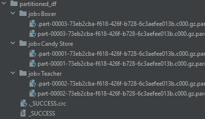
If you recall, the df2 DataFrame, has only 3 distinct values for the job column, hence 3 directories are created for each.
# Bucketing
df2.write.mode("overwrite").format("parquet").options(compression="gzip").bucketBy(2, "job").saveAsTable("sample_bucketized_df")

# The above command, saves the table in the `spark-warehouse` component. (No further details will be provided here)
# You can query the Hive table by the following commands:
spark.sql("SELECT * FROM sample_bucketized_df WHERE job=Boxer").show()
# +--------+-----+-----------+
# | user_id| name|        job|
# +--------+-----+-----------+
# |       1| Andy|Candy Store|
# ...
You can find a more detailed article on partitioning and bucketing here.
Some Useful Functions
from pyspark.sql.functions import countDistinct
# ============================================================
# To count the number of distinct (unique) values in each column

df3 = spark.createDataFrame(data=a + [(4, 'James', 'Teacher')], schema=strict_columns)
print(df3.collect())
# [Row(id=1, name='Andy', job='Candy Store'), Row(id=2, name='Julia', job='Teacher'), Row(id=3, name='Jamal', job='Boxer'), Row(id=4, name='James', job='Teacher')]
print(df3.select(countDistinct("job")).collect())
# [Row(count(DISTINCT job)=3)]
# ============================================================
from pyspark.sql.functions import spark_partition_id, collect_list
# ============================================================
# spark_partition_id: To filter/group based on the partition that the data is placed on
# collect_list: To aggregate corresponding columns into arrays

print(df3.groupBy(spark_partition_id().alias("pid")) \
         .agg(collect_list("id").alias("id_collection")) \
         .collect())
# [Row(pid=0, id_collection=[1]), Row(pid=1, id_collection=[2]), Row(pid=2, id_collection=[3]), Row(pid=3, id_collection=[4])]
# ============================================================
from pyspark.sql.functions import rand, randn
# ============================================================
# rand([seed]): Generates a random column with independent and identically distributed (i.i.d.) samples uniformly distributed in [0.0, 1.0).
# randn([seed]): Generates a column with independent and identically distributed (i.i.d.) samples from the standard normal distribution.

# If you pass a `seed` to either one of them, you can get a reproducible result
print(df3.where(randn() > 0.5).collect())
# [Row(id=3, name='Jamal', job='Boxer'), Row(id=4, name='James', job='Teacher')]
print(df3.where(randn() > 0.5).collect())
# []
print(df3.where(randn() > 0.5).collect())
# [Row(id=1, name='Andy', job='Candy Store')]
You can find the complete list of available PySpark SQL functions here.
Multiple Operations
# union
# ============================================================
# In order to append new rows or concat two DataFrames, we have to use the `union` method. Note that `union` doesn't check for schema mismatches:
print(df.union(df2).tail(2))
# [Row(user_id=3, name='Jamal', job='Boxer'), Row(user_id=None, name='JJJ', job='Manager')]

# Also, union is equal to SQL `UNION ALL`, so if you want to drop the duplicate records you should use `df.union(df2).distinct()`
Final Word
I hope this article provides a starting point as well as a reference for working with PySpark in a batch-processing approach. Real-time data will be covered in a later article as we take a look at Spark Structured Streaming module.
