

DataOps: Apache Spark - Basic
Apache Spark: A big data processing API
I'm a senior full-stack developer, and I love software engineering. I believe by working together we can create wonderful assets for the world, and we can shape the future as we shape our own destiny, and no goal is too ambitious. 💫 I try to be optimistic and energetic, and I'm always open to collaboration. 👥 Contact me if you have something on your mind and let's see where it goes 🚀
Introduction
Big data workloads are processed using Apache Spark, an open-source distributed processing engine. It uses efficient query execution and in-memory caching for quick analytic queries against any size of data. It offers code reuse across different workloads, including batch processing, interactive queries, real-time analytics, machine learning, and graph processing. Development APIs are available in Java, Scala, Python, and R. Apache Spark provides powerful libraries for many data processing operations such as:
MLlib
Spark includes MLlib, a library of algorithms to do machine learning on data at scale. The algorithms include the ability to do classification, regression, clustering, collaborative filtering, and pattern mining.
Spark Streaming
It ingests data in mini-batches and enables analytics on that data with the same application code written for batch analytics or streaming analytics. Spark Streaming supports data from Twitter, Kafka, Flume, HDFS, and ZeroMQ, and many others found in the Spark Packages ecosystem.
Spark SQL
A distributed query engine that provides low-latency, interactive queries up to 100x faster than (Hadoop's) MapReduce. It includes a cost-based optimizer, columnar storage, and code generation for fast queries while scaling to thousands of nodes.
GraphX
Provides ETL, exploratory analysis, and iterative graph computation to enable users to interactively build, and transform a graph data structure at scale.
(Source)
Descriptive Core Concepts
Clustered Architecture
Single machines do not have enough power and resources to perform computations on huge amounts of information (or the user probably does not have the time to wait for the computation to finish). A cluster, or group, of computers, pools the resources of many machines together, giving us the ability to use all the cumulative resources as if they were a single computer. Now, a group of machines alone is not powerful, you need a framework to coordinate work across them. Spark does just that, managing and coordinating the execution of tasks on data across a cluster of computers.
The cluster of machines that Spark will use to execute tasks is managed by a cluster manager like Spark’s standalone cluster manager, or YARN. We then submit Spark Applications to these cluster managers, which will grant resources to our application so that we can complete our work.
Spark Applications
Spark Applications consist of a driver process and a set of executor processes.
Driver
The driver process runs your main() function, sits on a node in the cluster, and is responsible for three things: maintaining information about the Spark Application; responding to a user’s program or input; and analyzing, distributing, and scheduling work across the executors.
Executors
Each executor is responsible for only two things: executing code assigned to it by the driver, and reporting the state of the computation on that executor back to the driver node.
Note
Though Spark is natively based on clustered operations, it can also run on one computing machine, called local mode. Which basically uses multi-threading processing to run the driver and executors.
Code-wise Core Concepts
Spark Session
You control your Spark Application through a driver process called the SparkSession, each Spark Application has one SparkSession. This variable can be accessed as spark in the interactive console.
DataFrames
A DataFrame is the most common Structured API and simply represents a table of data with rows and columns. The list that defines the columns and the types within those columns is called the schema. Natively, spark dataframes are partitioned across servers (clusters).
val sampleRange = spark.range(1000).toDF("number")
Partitions
Data is distributed in chunks called partitions across servers. A partition is a collection of rows that is on one physical machine in your cluster.
Transformations
In Spark, the core data structures are immutable, meaning they cannot be changed after they’re created. This might seem like a strange concept at first: if you cannot change it, how are you supposed to use it? To “change” a DataFrame, you need to instruct Spark how you would like to modify it to do what you want. These instructions are called transformations.
Transformations are the core of how you express your business logic using Spark. There are two types of transformations: those that specify narrow dependencies, and those that specify wide dependencies.
Narrow Transformations
Are those for which each input partition will contribute to only one output partition. Narrow transformations are:
Map
FlatMap
MapPartition
Filter (~ Where)
Sample
Union
Wide Transformations
Are those for which each input partition will contribute to many output partitions.
Intersection
Distinct
ReduceByKey
GroupByKey
Join
Cartesian
Repartition
Coalesce
// A Narrow Transformation:
val evens = sampleRange.where("number % 2 = 0")
After a wide transformation, Spark will write the results on different partitions, this is called shuffle, whereby Spark will exchange partitions across the cluster. With narrow transformations, Spark will automatically perform an operation called pipelining, meaning that if we specify multiple filters on DataFrames, they’ll all be performed in-memory. The same cannot be said for shuffles. When we perform a shuffle, Spark writes the results to disk.
Lazy Evaluation
Lazy evaluation means that Spark will wait until the very last moment to execute the graph of computation instructions. In Spark, instead of modifying the data immediately when you express some operation, you build up a plan of transformations that you would like to apply to your source data. This provides immense benefits because Spark can optimize the entire data flow from end to end.
Actions
Transformations allow us to build up our logical transformation plan. To trigger the computation, we run an action. There are three kinds of actions:
Actions to view data in the console
Actions to collect data to native objects in the respective language
Actions to write to output data sources
In Practice
DataFrames
For example, let's read some flight data from the US Bureau of Transportation provided by the official Spark documentation here.
//Read CSV and infer schema of the csv file.
scala> val flightData2015 = spark
  .read
  .option("inferSchema", "true")
  .option("header", "true")
  .csv("data/flight-data/csv/2015-summary.csv")

//The number of rows is unspecified because reading data is a transformation, and is therefore a lazy operation. To infer the schema, Spark peeks at the first few rows to try and guess the variable type of each column.

//Explain the execution plan of a sorting transformation
scala> flightData2015.sort("count").explain()
== Physical Plan ==
AdaptiveSparkPlan isFinalPlan=false
+- Sort [count#19 ASC NULLS FIRST], true, 0
   +- Exchange rangepartitioning(count#19 ASC NULLS FIRST, 200), ENSURE_REQUIREMENTS, [plan_id=33]
      +- FileScan csv [DEST_COUNTRY_NAME#17,ORIGIN_COUNTRY_NAME#18,count#19] Batched: false, DataFilters: [], Format: CSV, Location: InMemoryFileIndex(1 paths)[file:/Users/alirezasharifikia/dev/test/Spark/spark-3.3.2-bin-hadoop3/d..., PartitionFilters: [], PushedFilters: [], ReadSchema: struct<DEST_COUNTRY_NAME:string,ORIGIN_COUNTRY_NAME:string,count:int>

// No need to fully understand the above command for now.

// By default, spark uses 200 partitions for each shuffle operation, so let's reduce that:
scala> spark.conf.set("spark.sql.shuffle.partitions", "5")

// Execute the transformation by `take` action
scala> flightData2015.sort("count").take(2)
res5: Array[org.apache.spark.sql.Row] = Array([United States,Singapore,1], [Moldova,United States,1])
The execution process for the last command would be something like this:
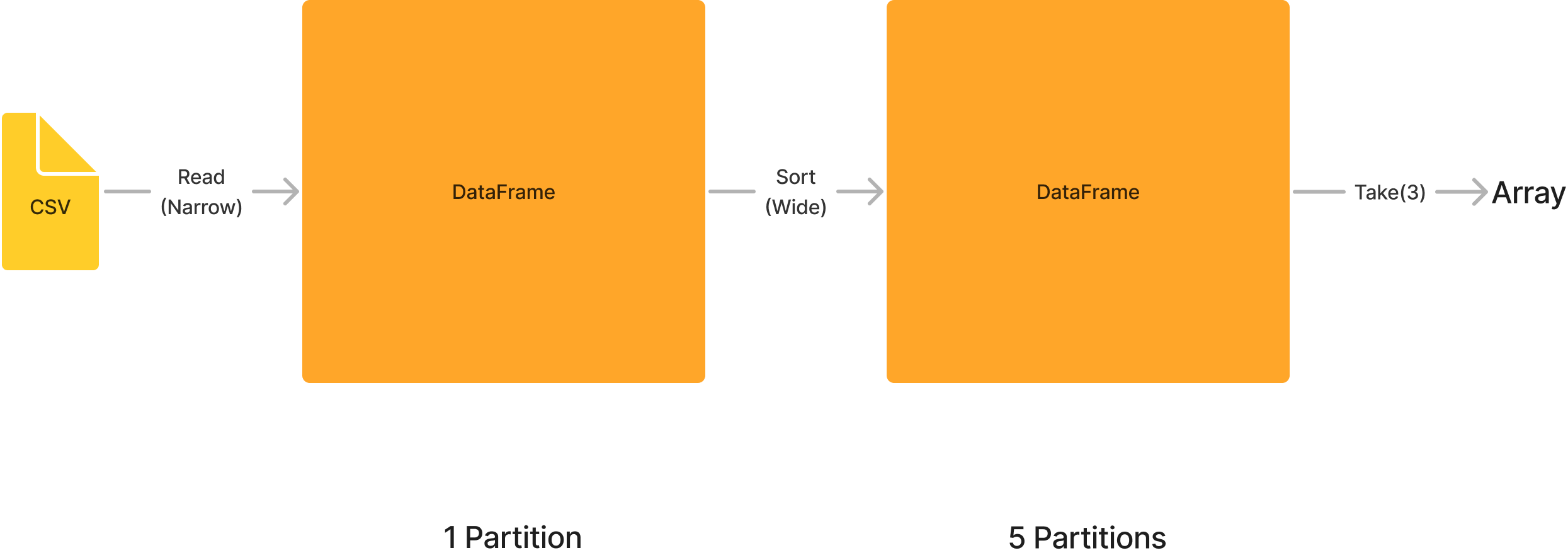
The logical plan of transformations that we build up defines a lineage for the DataFrame so that at any given point in time, Spark knows how to recompute any partition by performing all of the operations it had before on the same input data. This sits at the heart of Spark’s programming model— functional programming where the same inputs always result in the same outputs when the transformations on that data stay constant.
DataFrames & SQL
With Spark SQL, you can register any DataFrame as a table or view (a temporary table) and query it using pure SQL. There is no performance difference between writing SQL queries or writing DataFrame code, they both “compile” to the same underlying plan that we specify in DataFrame code.
You can make any DataFrame into a table or view with one simple method call:
flightData2015.createOrReplaceTempView("flight_data_2015")
Now in order to use SQL we can write the following code
scala> val sqlWay = spark.sql("""
SELECT DEST_COUNTRY_NAME, count(1)
FROM flight_data_2015
GROUP BY DEST_COUNTRY_NAME
""")

scala> val dataFrameWay = flightData2015
  .groupBy('DEST_COUNTRY_NAME)
  .count()

scala> sqlWay.explain
== Physical Plan ==
AdaptiveSparkPlan isFinalPlan=false
+- HashAggregate(keys=[DEST_COUNTRY_NAME#17], functions=[count(1)])
   +- Exchange hashpartitioning(DEST_COUNTRY_NAME#17, 5), ENSURE_REQUIREMENTS, [plan_id=55]
      +- HashAggregate(keys=[DEST_COUNTRY_NAME#17], functions=[partial_count(1)])
         +- FileScan csv [DEST_COUNTRY_NAME#17] Batched: false, DataFilters: [], Format: CSV, Location: InMemoryFileIndex(1 paths)[file:/Users/alirezasharifikia/dev/test/Spark/spark-3.3.2-bin-hadoop3/d..., PartitionFilters: [], PushedFilters: [], ReadSchema: struct<DEST_COUNTRY_NAME:string>


scala> dataFrameWay.explain
== Physical Plan ==
AdaptiveSparkPlan isFinalPlan=false
+- HashAggregate(keys=[DEST_COUNTRY_NAME#17], functions=[count(1)])
   +- Exchange hashpartitioning(DEST_COUNTRY_NAME#17, 5), ENSURE_REQUIREMENTS, [plan_id=68]
      +- HashAggregate(keys=[DEST_COUNTRY_NAME#17], functions=[partial_count(1)])
         +- FileScan csv [DEST_COUNTRY_NAME#17] Batched: false, DataFilters: [], Format: CSV, Location: InMemoryFileIndex(1 paths)[file:/Users/alirezasharifikia/dev/test/Spark/spark-3.3.2-bin-hadoop3/d..., PartitionFilters: [], PushedFilters: [], ReadSchema: struct<DEST_COUNTRY_NAME:string>
If you inspect the explain output, you'll notice that there's no difference for Spark which way you choose. Also, when you use spark.sql(...) you'll get returned a DataFrame, so one can flexibly write their own logic however one might want at any given point.
More Complex Queries
SQL way:
val maxSql = spark.sql("""
SELECT DEST_COUNTRY_NAME, sum(count) as destination_total
FROM flight_data_2015
GROUP BY DEST_COUNTRY_NAME
ORDER BY sum(count) DESC
LIMIT 5
""")

+-----------------+-----------------+
|DEST_COUNTRY_NAME|destination_total|
+-----------------+-----------------+

scala> maxSql.explain
== Physical Plan ==
AdaptiveSparkPlan isFinalPlan=false
+- TakeOrderedAndProject(limit=5, orderBy=[destination_total#63L DESC NULLS LAST], output=[DEST_COUNTRY_NAME#17,destination_total#63L])
   +- HashAggregate(keys=[DEST_COUNTRY_NAME#17], functions=[sum(count#19)])
      +- Exchange hashpartitioning(DEST_COUNTRY_NAME#17, 5), ENSURE_REQUIREMENTS, [plan_id=116]
         +- HashAggregate(keys=[DEST_COUNTRY_NAME#17], functions=[partial_sum(count#19)])
            +- FileScan csv [DEST_COUNTRY_NAME#17,count#19] Batched: false, DataFilters: [], Format: CSV, Location: InMemoryFileIndex(1 paths)[file:/Users/alirezasharifikia/dev/test/Spark/spark-3.3.2-bin-hadoop3/d..., PartitionFilters: [], PushedFilters: [], ReadSchema: struct<DEST_COUNTRY_NAME:string,count:int>

scala> maxSql.show()
+-----------------+-----------------+
|DEST_COUNTRY_NAME|destination_total|
+-----------------+-----------------+
|    United States|           411352|
|           Canada|             8399|
|           Mexico|             7140|
|   United Kingdom|             2025|
|            Japan|             1548|
+-----------------+-----------------+
DataFrame way:
scala> import org.apache.spark.sql.functions.desc
scala> flightData2015
  .groupBy("DEST_COUNTRY_NAME")
  .sum("count")
  .withColumnRenamed("sum(count)", "destination_total")
  .sort(desc("destination_total"))
  .limit(5)
  .show()
+-----------------+-----------------+
|DEST_COUNTRY_NAME|destination_total|
+-----------------+-----------------+
|    United States|           411352|
|           Canada|             8399|
|           Mexico|             7140|
|   United Kingdom|             2025|
|            Japan|             1548|
+-----------------+-----------------+
The execution plan would be something like the following. These representations are called Directed Acyclic Graph (DAG) and the result of each step is a new immutable DataFrame.

Final Word
I'm going to conclude the introduction to Apache Spark here. I might write more about it in the future. In the next article, we'll be covering Apache Kafka.
