

Enterprise Level Machine Learning Tools & Tips: Part 4: Regression vs Classification
Understanding Methods, Strengths, and Limitations

I'm a senior full-stack developer, and I love software engineering. I believe by working together we can create wonderful assets for the world, and we can shape the future as we shape our own destiny, and no goal is too ambitious. 💫 I try to be optimistic and energetic, and I'm always open to collaboration. 👥 Contact me if you have something on your mind and let's see where it goes 🚀
Introduction
Machine learning encompasses a wide range of techniques and algorithms that enable computers to learn patterns from data and make predictions or decisions. Two fundamental problem types in machine learning are:
Regression: the goal is to predict continuous numerical values
Classification: the aim is to assign data points to discrete categories or classes.
This article provides an overview of these problem types and introduces some popular methods used in regression and classification tasks, along with their strengths and weaknesses.
| Condition | Regression | Classification |
| Label Data Type | Numeric | Categorical |
| Problem is | Ordinal | Non-ordinal |
| Label Domain | Real Numbers | Discrete Numbers |
| Evaluation Metrics | Error-Related (RMSE, etc.) | Performance-Related (Accuracy, etc.) |
Regression
Regression is the process of finding a function for modeling the pattern of ordinal data. Finding a solution for regression problems requires extensive knowledge about how the features (input) correlate to the label(s) (output). Based on this relationship you could go with Linear Regression or Polynomial Regression techniques.
Linear Regression
This is used to model a linear relationship between the feature(s) and a label:
$$y = a_0 + a_1x_1 + a_2x_2 + ...$$
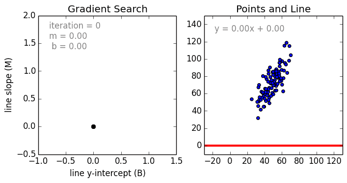
The weight training (learning) process is performed by Stochastic Gradient Descent (SGD), which is an iterative process of updating weights based on the learning rate and loss function (which is dependent on the value of each weight).
The process can be visualized like this:
(Source)
Pros
Simplicity: Linear regression is a simple and straightforward algorithm, making it easy to understand and implement.
Interpretability: Linear regression provides interpretable coefficients that indicate the direction and magnitude of the relationship between the input features and the target variable. This allows for easy interpretation and understanding of the impact of each feature on the outcome. Larger coefficients indicate a stronger influence on the target variable, helping identify the most influential features.
Fast Inference: After training is done, is very efficient for real-time or time-sensitive applications.
Assumptions and Diagnostics: Linear regression has well-defined assumptions and diagnostic tools to assess model performance and check for violations of assumptions, such as linearity, independence, and homoscedasticity.
Cons
Linearity Assumption: Linear regression assumes a linear relationship between the input features and the target variable, especially if the relationship is non-linear.
Sensitivity to Outliers: Linear regression can be sensitive to outliers, as the least squares method used for optimization aims to minimize the sum of squared errors. Outliers can have a disproportionate impact on the model's performance.
Assumptions and Violations: Violations of linear regression assumptions, such as heteroscedasticity or multicollinearity, can affect the model's accuracy and interpretation. These violations need to be addressed to ensure reliable results.
Limited Performance on Non-linear Data: For non-linear relationships, more advanced regression techniques, like [polynomial regression](https://www.analyticsvidhya.com/blog/2021/10/understanding-polynomial-regression-model/#:~:text=Polynomial%20regression%2C%20abbreviated%20E(y,the%20variance%20of%20the%20coefficients.) or decision tree regression, may be more appropriate.
Decision Tree Regression
Uses a decision tree structure to make predictions. Here's how it works:
Building the Tree: The decision tree is constructed by recursively partitioning the feature space based on the input features. The goal is to create homogeneous subsets of data at each node, optimizing for reduced variance or squared error in the target variable.
Splitting Criteria: The decision tree determines the best feature and split point at each node using criteria such as mean squared error, variance reduction, or Gini impurity. The splits are chosen to maximize the homogeneity of the target variable within each resulting subset.
Prediction: Once the tree is constructed, predictions are made by traversing the tree from the root node to a leaf node. At each node, the appropriate branch is chosen based on the feature values of the input, until a leaf node is reached. The predicted value at the leaf node is then used as the output.
Note: There are no explicit weights as in some other algorithms like linear regression. Instead, the algorithm focuses on partitioning the feature space based on feature thresholds and creating rules for predictions. The splits and thresholds are determined during the training process based on the optimization criteria specific to decision tree regression.
Pros
Interpretable: Decision trees provide clear insights into feature importance and decision-making, making them easy to interpret and explain.
Non-linear Relationships: Decision trees can capture non-linear relationships between features and the target variable effectively.
Handling Missing Values: Decision trees can handle missing values by utilizing surrogate splits and imputing missing data.
Robust to Outliers: Decision trees are robust to outliers as they partition the feature space based on thresholds and are not affected by extreme values.
Cons
Overfitting: Decision trees are prone to overfitting, capturing noise or irrelevant patterns in the data. Techniques like pruning or ensembling can be used to mitigate this issue.
Instability: Small changes in the data can lead to different tree structures, resulting in instability.
Lack of Smoothness: Decision tree predictions can be discontinuous, leading to step-like patterns rather than smooth curves.
Difficulty Capturing Linear Relationships: Decision trees may struggle to capture linear relationships effectively compared to linear regression algorithms.
Random Forest Regression
Combines multiple decision trees to make predictions. Here's how it works:
Building the Forest: Random Forest Regression involves constructing an ensemble of decision trees. Each tree is built using a random subset of the training data and a random subset of features. This randomness introduces diversity and reduces overfitting.
Training the Trees: Each decision tree in the forest is trained on a different subset of the data using a process similar to traditional decision tree regression. The trees are grown by recursively partitioning the feature space based on the input features and minimizing the variance or mean squared error of the target variable.
Aggregating Predictions: During the prediction phase, each tree in the forest independently predicts the target variable based on the input features. The final prediction is obtained by aggregating the predictions from all the trees, typically through averaging.
Note: Weights are not explicitly updated in Random Forest Regression. Instead, the algorithm focuses on building a collection of decision trees, each trained on different subsets of the data and features. The predictions of individual trees are combined using averaging or voting to obtain the final prediction.
Pros
Improved Predictive Accuracy: Random Forest Regression tends to have higher predictive accuracy compared to individual decision trees, as it mitigates the risk of overfitting by averaging predictions from multiple trees.
Robust to Outliers and Noise: Random Forest Regression is robust to outliers and noisy data since individual trees are less affected by individual instances due to the averaging effect.
Non-linear Relationships: Random Forest Regression can capture non-linear relationships and complex interactions between features, making it effective for modeling complex data patterns.
Feature Importance: Random Forest Regression provides a measure of feature importance based on how much each feature contributes to the overall prediction accuracy. This helps identify the most influential features.
Cons
Complexity: Random Forest Regression is more complex than individual decision tree models, making it computationally expensive and requiring more resources for training and prediction.
Lack of Interpretability: The ensemble nature of Random Forest Regression makes it less interpretable than a single decision tree. It may be challenging to explain the specific impact of each feature on the target variable.
Hyperparameter Tuning: Random Forest Regression has several hyperparameters that need to be tuned to achieve optimal performance. This tuning process can be time-consuming and requires careful experimentation.
Q: How can random forest regression both have a strong point in Feature Importance and a negative point in Lack of Interpretability?
A: Random forest regression's feature importance provides a broader understanding of the relative significance of features within the model. However, due to the ensemble structure and the interactions among the trees, explaining the exact relationship between a specific feature and a particular prediction becomes more challenging, leading to the perceived lack of interpretability.
Classification
Classification is the process of finding the probability of a target belonging to single or multiple classes.
Binary Classification
When the problem is about whether a subject belongs to a class (1) or not (0), it has 2 outcomes.
Multiclass Classification
When the number of available classes is more than 2.
Hierarchical Classification
It allows for classification at multiple levels of granularity, where classes at lower levels inherit characteristics from higher-level classes. This is useful when the classes have a natural hierarchical relationship.
One-vs-One Classification
Splits a multi-class classification into one binary classification problem per class. For example, consider a classification problem for which we're trying to find out if a photo belongs to a cat, a dog, a bird, or a horse. For this matter, the following models are then created:
Model 1: cat vs dog
Model 2: cat vs horse
Model 3: cat vs bird
Model 4: dog vs horse
Model 5: dog vs bird
Model 6: horse vs bird
The number of required classes is calculated by the following combination:
$$\binom {Number\ of\ Labels} 2 = \frac{Labels!}{2!(Labels - 2)!}$$
Which would be a serious issue in classification problems with a large number of classes.
Then the models are trained on the same dataset (to give equal learning chances) and then the prediction (classification) has to be performed by all the models. The winner would then be calculated by the maximum probability.
Methods
Neural Networks with Softmax Output Layer: Neural networks can be used for one-vs-one classification by using a softmax output layer. Each node in the output layer represents a class, and the softmax function converts the outputs into probabilities. During prediction, the class with the highest probability is selected as the final prediction.
DAGSVM (Directed Acyclic Graph Support Vector Machines): DAGSVM constructs a directed acyclic graph where each node represents a binary classifier. The graph structure reflects the relationships between the classes. Each classifier is trained to distinguish between two connected classes in the graph. During prediction, the input sample traverses the graph, and the final prediction is made based on the path taken.
One-vs-Many Classification
Splits a multi-class classification into one binary classification problem per each pair of classes. Basically, one model is created per class and is compared against others. For the same example above, the following models are created:
Model 1: cat vs [dog, horse, bird]
Model 2: dog vs [cat, horse, bird]
Model 3: horse vs [cat, dog, bird]
Model 4: bird vs [cat, dog, horse]
The number of required classes is equal to the number of labels.
Then the models are trained on the same dataset (to give equal learning chances) and then the prediction (classification) has to be performed by all the models. The model with the highest metric is deemed the winner.
Methods
Logistic Regression: Multiple binary classifiers are trained, each distinguishing between one class and the rest of the classes. It assumes a linear relationship between features and the logarithm of the odds, which might not capture complex nonlinear relationships.
Support Vector Machines (SVM): Multiple binary classifiers are trained, each distinguishing between one class and the rest of the classes.
Neural Networks with Softmax Output Layer: Each node in the output layer represents a class, and the softmax function converts the outputs into probabilities. During prediction, the class with the highest probability is selected as the final prediction.
Diving Deeper
Let's take a closer look at some of the introduced methods in the Classification section of this article.
Logistic Regression
It's a popular statistical and machine-learning algorithm used for binary classification. Here's an overview of how it works:
Logistic Function (Sigmoid): Logistic Regression utilizes the logistic function, also known as the sigmoid function, to model the relationship between the input features and the binary target variable. The sigmoid function maps any real-valued number to a value between 0 and 1, representing the probability of the instance belonging to the positive class.
Hypothesis Representation: Logistic Regression assumes a linear relationship between the input features and the logarithm of the odds (log-odds) of the positive class. The hypothesis function calculates the log-odds, which is then transformed using the sigmoid function to obtain the predicted probability.
Training and Weights: During training, Logistic Regression learns the optimal weights (coefficients) that minimize the difference between the predicted probabilities and the actual binary labels. This is typically achieved through optimization algorithms such as gradient descent or Newton's method, which iteratively update the weights based on the gradients of the cost function.
Decision Boundary: Once the weights are learned, Logistic Regression can classify new instances by evaluating the hypothesis function and applying a threshold (usually 0.5). If the predicted probability is above the threshold, the instance is classified as the positive class; otherwise, it is classified as the negative class.
Popular Applications
Predicting whether an email is spam or not.
Diagnosing diseases based on medical test results.
Assessing the likelihood of customer churn in a subscription service.
Analyzing credit risk to determine the probability of default.
Pros
Simplicity: Logistic Regression is relatively simple and easy to understand, making it accessible to both beginners and experts.
Interpretable: The coefficients of the logistic regression model represent the influence and directionality of each feature, allowing for interpretability and insights into feature importance.
Fast Training and Prediction: Logistic Regression is computationally efficient and scales well to large datasets, enabling fast training and prediction.
Handles Irrelevant Features: Logistic Regression can handle datasets with irrelevant or redundant features without significantly impacting its performance.
Cons
Linear Assumption: Logistic Regression assumes a linear relationship between the features and the log-odds of the positive class. It may not capture complex nonlinear relationships between features and the target variable.
Limited Complexity: Logistic Regression may not be suitable for tasks with intricate decision boundaries or highly complex data patterns that cannot be adequately approximated by a linear model.
Susceptible to Outliers: Logistic Regression can be sensitive to outliers, which can have a disproportionate impact on the model's performance.
Imbalanced Classes: Logistic Regression may struggle with imbalanced datasets where the number of instances in each class is significantly different. Techniques such as class weighting or resampling can help address this issue.
SVM
It's a powerful supervised machine learning algorithm used for both classification and regression tasks. Here's an overview of how SVM works:
Margin Maximization: SVM aims to find the optimal hyperplane that separates the instances of different classes with the largest possible margin. The margin is the distance between the hyperplane and the closest instances of each class, known as support vectors.
Kernel Trick: SVM can efficiently handle linearly inseparable data by applying the kernel trick. It transforms the input features into a higher-dimensional space, where the instances become linearly separable. This allows SVM to find nonlinear decision boundaries.
Support Vectors: The support vectors are the instances closest to the decision boundary. These instances have the most influence on determining the position and orientation of the hyperplane. Only the support vectors are used in the weight computation, making SVM memory-efficient.
Weight Optimization: The weights in SVM are updated during training to find the optimal hyperplane. The objective is to maximize the margin while minimizing the classification errors. This is typically achieved through convex optimization techniques, such as quadratic programming.
Popular Applications
Text categorization and sentiment analysis.
Image classification and object recognition.
Bioinformatics for gene expression analysis.
Fraud detection and anomaly detection.
Pros
Effective in High-Dimensional Spaces: SVM performs well in high-dimensional feature spaces, making it suitable for problems with a large number of features.
Robust to Overfitting: SVM is less prone to overfitting, as it maximizes the margin and focuses on the instances near the decision boundary.
Versatility: SVM supports various kernel functions, such as linear, polynomial, radial basis function (RBF), and sigmoid. This flexibility allows it to handle different types of data and capture complex relationships.
Works well with Small to Medium-Sized Datasets: SVM performs well with small to medium-sized datasets. It is memory-efficient because it only relies on the support vectors.
Cons
Computational Complexity: SVM can be computationally expensive, especially for large datasets and complex kernel functions. Training time and memory requirements can increase significantly.
Parameter Sensitivity: SVM has several hyperparameters, such as the choice of kernel, regularization parameter (C), and kernel-specific parameters. Selecting appropriate values for these parameters is crucial for optimal performance.
Lack of Interpretability: SVM models are not easily interpretable. The resulting hyperplane may not directly correspond to meaningful interpretations of the original features.
Limited Scalability: SVM's training time and memory usage can become prohibitive for very large datasets. Specialized techniques like stochastic gradient descent or kernel approximation methods can be used to mitigate this issue.
Neural Networks (ANN)
Learn about the key differences between regression and classification in machine learning. Explore various methods such as linear regression, logistic regression, support vector machines (SVM), and neural networks. Understand the pros and cons of each method and how they work, empowering you to choose the right approach for your problem.
Also known as Artificial Neural Networks (ANN), are a class of machine learning models inspired by the structure and functioning of biological neural networks in the human brain. Here's an overview of how neural networks work:
Structure: A neural network consists of interconnected layers of artificial neurons, called nodes or units. The layers include an input layer, one or more hidden layers, and an output layer. Each node takes inputs, performs computations, and produces an output signal.
Feedforward Propagation: The input signals are propagated forward through the network, layer by layer, in a process called feedforward propagation. The outputs of one layer serve as inputs to the next layer, with weights assigned to the connections between the nodes.
Activation Function: Each node applies an activation function to the weighted sum of its inputs, introducing nonlinearity to the model. Common activation functions include sigmoid, ReLU (Rectified Linear Unit), and tanh.
Weighted Sum and Bias: Each connection between nodes has an associated weight, which determines the strength of the connection. Additionally, each node typically has a bias term that provides an offset to the weighted sum.
Training and Weight Updates: Neural networks are trained through a process called backpropagation. During training, the network's output is compared to the desired output, and the error is propagated backward through the network to adjust the weights. Optimization algorithms, such as gradient descent, are used to update the weights iteratively.
Popular Applications
Image and speech recognition.
Natural language processing.
Recommendation systems.
Time series forecasting.
Autonomous vehicles.
Pros
Nonlinear Modeling: Neural networks can capture complex, nonlinear relationships between features and target variables, making them effective for tasks with intricate patterns.
Universal Approximators: Neural networks have the capacity to approximate any continuous function, given sufficient resources and appropriate architecture.
Feature Learning: Neural networks can automatically learn relevant features from raw or high-dimensional data, reducing the need for manual feature engineering.
Parallel Processing: Neural networks can be highly parallelized, taking advantage of modern GPU architectures and distributed computing to expedite training and inference.
Cons
Computational Complexity: Training neural networks can be computationally expensive, particularly for large and deep architectures. Extensive computing resources and time are often required.
Black Box Nature: The inner workings of neural networks can be complex and difficult to interpret, limiting the transparency and interpretability of the model.
Overfitting: Neural networks are susceptible to overfitting, where the model learns to memorize the training data instead of generalizing well to unseen data. Regularization techniques and proper validation are needed to mitigate this.
Data Requirements: Neural networks typically require a large amount of labeled data to generalize effectively. Insufficient training data may lead to poor performance.
Final Note
I hope this article has provided you with valuable insights into the problem definition in machine learning. It's crucial to dive deeper into each topic and explore the methods in more detail based on your specific needs and datasets. Remember, there is always more to learn and discover in the exciting field of machine learning.
In a future article, we will delve into the fascinating world of deep learning. Until then, happy researching, and may your machine-learning endeavors be successful.