

Enterprise Level Machine Learning Tools & Tips: Part 1
Part 1: Data Analysis and Model Evaluation Techniques.
I'm a senior full-stack developer, and I love software engineering. I believe by working together we can create wonderful assets for the world, and we can shape the future as we shape our own destiny, and no goal is too ambitious. 💫 I try to be optimistic and energetic, and I'm always open to collaboration. 👥 Contact me if you have something on your mind and let's see where it goes 🚀
For those who are familiar with machine learning, I'm going to describe multiple topics that one faces while implementing enterprise-level AI. I'm going to list and explain some of the available tools from statistical analysis methods, to the mathematics involved, and my experience as a professional developer.
Data Analysis
Statistical: Descriptive Statistics
Central Tendencies
Mode
The most common value in the dataset.
Mean
In statistics, average is called mean.
$$mean(x) = \bar{x} = \frac{\Sigma(x_i)}{n}$$
Median
The middle point of a sorted ordinal dataset.
For example, in a normal distribution mean = mode = median and skewness = 0 (I'll introduce it a bit later).
Dispersion
Range
Minimum and maximum of the dataset. You can use these values to handle outliers, for example by setting the NaN values to the maximum range of the Dataset.
Variance
A parameter representing the spread of the dataset.
$$Variance(x)=\sigma^2=\frac{\Sigma (x - \bar{x})^2}{n}$$
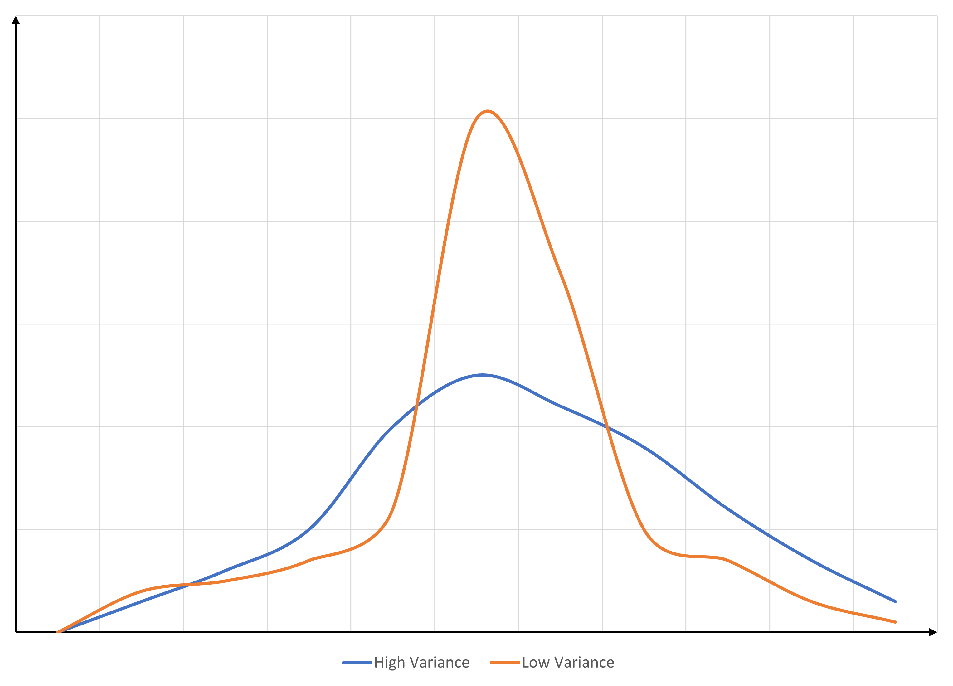
Standard Deviation
Shows how far away we are from the mean of the dataset.
$$\sqrt{Variance(x)}=\sigma$$
Distribution
Skenewss
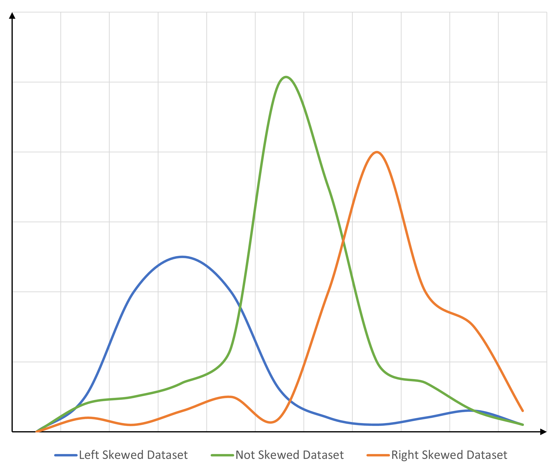
Kurtosis
How is the distribution in comparison with a normal distribution?
Right-skewed datasets have a positive kurtosis, while left-skewed datasets have a negative kurtosis.
Positive kurtosis is an indicator of the fact that the mean and median of the dataset are lower than those of an imaginary normal distribution, whereas negative kurtosis indicates the opposite.
Practical: Oversampling vs Undersampling
The Problem
Especially in classification problems, when the distribution of data for each class is imbalanced, the model's classification precision for data classes that belong to the minority class will be severely impacted, and this will lead to biased learning.
The Solution
To give the model a fair chance in learning the features of those minorities as well as other classes, one of the techniques is to decrease the training data for the majority class. This is called Undersampling. There are 3 techniques mentioned by MastersInDataScience.org that I follow based on the use case:
In the first technique, they keep events from the majority class that have the smallest average distance to the three closest events from the minority class on a scatter plot.
In the second, they use events from the majority class that have the smallest average distance to the three furthest events from the minority class on a scatter plot.
In the third, they keep a given number of majority class events for each event in the minority class that are closest on the scatter plot.
Another way to solve the issue is to Oversample the minority class, in which the size of rare transactions is increased.
Tips
Never undersample nor oversample the validation and holdout (test) datasets. For the evaluation of the model to have a meaningful result, the holdout dataset needs to represent near real-world data and so the data distribution should stay intact.
Both of the techniques can be used in the analysis and ETL (Extract, Transform, Load) phase to balance out the whole dataset; however, it's important to know where to use them. If the ratio of the majority to minority class is 1,000:1 then the model might lose some important trends and learning opportunities if you were to undersample the majority class. In these situations, it's better to oversample the minority rather than discard a significant amount of data from the majority class.
After either one of these techniques, the sampled data class needs to be reevaluated and checked for biases and a valid distribution of features must be ensured.
Evaluation Metrics
Confusion Matrix
One of the key concepts of an ML model performance evaluation is the TP, TN, FP, and FN metrics, which are True Positive, True Negative, False Positive, and False Negative. The concept is rather simple but I tend to look it up online every time because it's easy to get lost in words, so I'm going to leave a comprehensive and easy visual guide here:
Example
Imagine visiting a palm reader and they start foreseeing your future. Later in your life, if you want to evaluate the performance of the foreteller based on the events you've experienced, you can use the following figure called Confusion Matrix:
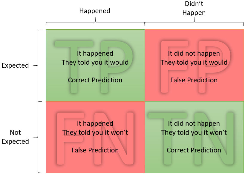
In machine learning, all of these metrics can be used to describe the performance of the model, and based on these rates, some other more complex criteria are calculated and further analyzed.
Based on the value of these occurrences, the following metrics are defined:
$$TPR: Sensitivity = \frac{TP}{TP + FN} = \frac{Correct\ Positive\ Predictions}{Total\ Expected\ Predictions}$$
$$FPR: Fall-Out = \frac{FP}{FP + TN} = \frac{False\ Positive\ Predictions}{Total\ Unexpected\ Predictions}$$
$$TNR: Specificity \ (Selectivity) = \frac{TN}{TN + FP} = \frac{Correct\ Negative\ Predictions}{Total\ Unexpected\ Predictions}$$
$$FNR: Miss-Rate = \frac{FN}{FN + TP} = \frac{False\ Negative\ Predictions}{Total\ Expected\ Predictions}$$
Tip
The confusion matrix, although confusing, is considered to be suitable for presenting data to stakeholders and non-technical members. It's best to equip the presentation with proper guidance and materials for disclosing these metrics.
An important criterion, complementary to the topic at hand is:
ROC
ROC stands for Receiver Operating Characteristic Curve that graphs the TPR vs FPR and allows us to compute a significant metric called AUC ROC which is the calculated Area Under the Curve of ROC as shown below:
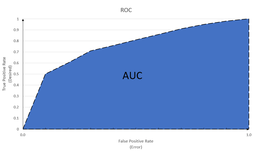
If we pay attention to the formulae provided in the last section, we'll notice that all four metrics of the last section are included in plotting TPR vs FPR. So this chart provides a powerful tool to measure the model's performance across all the provided metrics. To put the matter into better wording, I'm burrowing the phrasing of AnalyticsIndiaMag.com:
AUC-ROC is the valued metric used for evaluating the performance in classification models. The AUC-ROC metric clearly helps determine and tell us about the capability of a model in distinguishing the classes. The judging criteria being - Higher the AUC, better the model. AUC-ROC curves are frequently used to depict in a graphical way the connection and trade-off between sensitivity and
specificity(fall-out) for every possible cut-off for a test being performed or a combination of tests being performed. The area under the ROC curve gives an idea about the benefit of using the test for the underlying question.
Tips
The most significant benefit of ROC is that it can show the performance of the model independent of the classification threshold.
But, that's not always a desirable outcome. Because sometimes the cost of classification is too high, and we would like to focus on minimizing/maximizing one metric; for example, when trying to identify rotten eggs by an AI, no false negatives must happen because it might lead to health issues for the consumers.
This is NOT a good metric for presenting the performance of the model to the business stakeholders because it needs a technical background and also, since the classification threshold is of utmost importance in most cases of implementing a machine learning solution on an enterprise level, this tool is not recommended.
Accuracy
Calculated from the Confusion Matrix, accuracy is defined as follows:
$$Accuracy = \frac{TP + TN}{TP + TN + FP + FN} = \frac{Correct\ Predictions}{Total\ Predictions}$$
Accuracy as a metric is the best match for a use case with discrete and balanced labels; however, usually, accuracy alone is not a good metric for evaluating the model's performance, since most datasets are imbalanced. Consider the following examples:
Example #1
Consider a model that can predict if a person can pick the winning ticket out of a raffle with a size of 100, with a 3% accuracy. Is this model considered to be good?
If one were to randomly select the winner, one has a chance of 1% so this model has 3 times more chance to select the winner. It's definitely an improvement.
Example #2
Consider an ML that out of a dataset with a size of 100, the evaluation results in 80 TPs, 4 TNs, 13 FPs, and 3 FNs. This results in an (80 + 4)/100 accuracy which is quite good at first glance but it results in 13 subjects being labeled erroneous as positive while the number of results that were correctly labeled as negative is only 4.
To address this issue, two other metrics are considered:
Precision vs Recall
Precision is defined as "What portion of positive predictions was actually correct?"
Recall is defined as "What portion of positive records was predicted correctly?"
In mathematical terms:
$$Precision = \frac{TP}{TP + FP} = \frac{Correct\ Positive\ Predictions}{Total\ Positive\ Predictions}$$
$$Recall = \frac{TP}{TP + FN} = \frac{Correct\ Positive\ Predictions}{Total\ Positive\ Records}$$
Tips
In real-world examples, precision and recall have an opposite relationship with the classification threshold. Precision might increase as the acceptable threshold is increased (gets more strict) while recall might decrease; because less positive edge cases will be labeled as positive by the model.
Depending on the goal of the ML and mislabeling cost, often times one might have to be sacrificed for the other. For example, if mislabeling has devastating costs for the company, one must prioritize Precision, but if one would like to model to identify as many cases as possible and the mislabeling will NOT result in serious drawbacks, one might consider increasing Recall.
Precision and Recall are considered suitable metrics when working with imbalanced datasets.
F₁-Score
F₁-score is a measure of a test's success. In ML usually, only the F₁ score is considered and it's an aggregated metric by which one can evaluate the precision and recall together. The formula is as follows:
$$F_1 = \frac{2}{Precision^{-1} + Recall^{-1}}$$
Generally, the higher F₁ score is, the model is considered to be performing better.
Tip
This is NOT a good metric for presenting the performance of the model to the business stakeholders because it needs a mathematical and technical background; also if there's an imbalance in the cost of mislabeling for each class of the dataset, it's important to consider precision and recall separately while considering the mislabeling cost for the company.
Final Word
I'm going to end Part 1 here and introduce more advanced subjects and explore some of GCP stacks in the next parts of my ML series. If you find this interesting, have a comment, or think a section needs more explanation, reach out to me and I'll do my best to be responsive.
